TECTONICS BLOG Rev

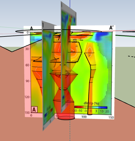
Click on an image to enlarge it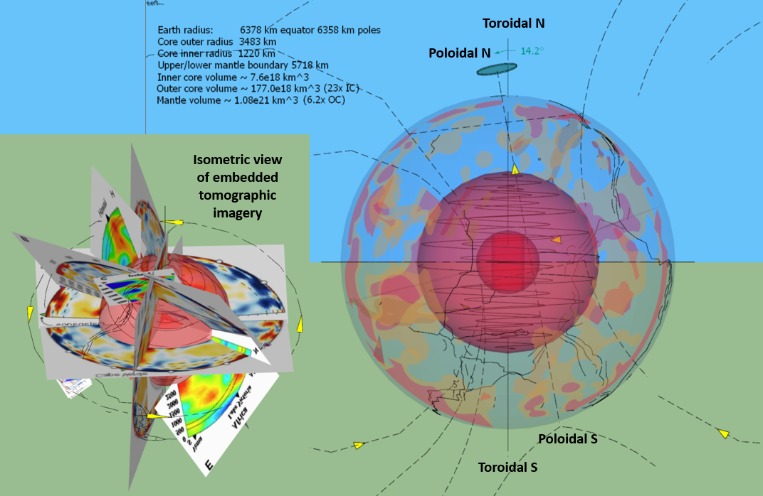

Figure 1. The geomagnetic field equipotential lines mapped over time showing wander of Earth's geomagnetic field over the past four centuries. The rate of polar drift has increased over the past decade. It appears that Earth has four magnetic poles, one set of which is relatively fixed, and another more subject to wander. This quadrapolar field currently has two poles in the North that are nearly convergent but another two in the South that are diverging. The fixed set is aligned with the planetary spin axis and may represent the toroidal component generated in the outer core. The other wandering set is likely the poloidal component generated from spinning mantle structures.

SketchUp Pro model of Earth

Figure 2. Screen captures of the SUP model of Earth's structural layers and 16 embedded seismic-tomographic images portraying mantle structure. The total-field electrical components are shown to the right and include both a toroidal and poloidal dipole components that combine into Earth's quadrapolar total field.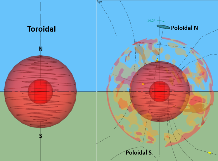

Model Components of Earth's Geodynamo

Figure 3. Details of the SUP model showing differentiated model components . The toroidal field is generate in the outer core with hydrodynamic stimulation from planetary spin. That dipole is fixed on the spin axis in agreement with computer model showing electromagnetic activity focused along the spin axis in the outer core. The poloidal field is more variable and in perpetual flux because its generated by a heterogeneous mantle subject to internal and external stimulation from both plate tectonics and impact tectogenesis.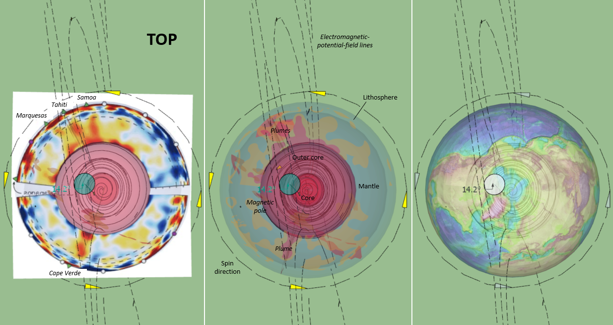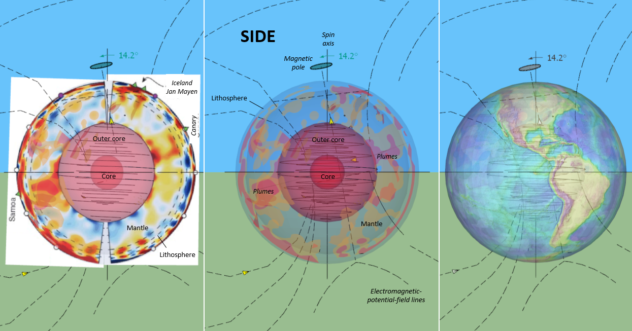

SketchUp Pro model of Earth

Figure 4. Top (above) and Side (below) views of an Earth SketchUp Pro model showing embedded seismic-wave (P- wave) tomography slices of the mantle (left). The model includes mantle plumes corresponding to the slowest-transmitting regions that are shaded red with surrounding slower ones shown in orange. The exact nature of the mantle heterogeneity is speculative, but the hottest and slowest-transmitting regions likely involving diffusion creep with localized magma generation and ascent. An array of plumes and colder, ferrous, mantle structures are electrically connected to the core where circulating Fe-rich magma surrounding a solid, ferrous core generate our electromagnetic field.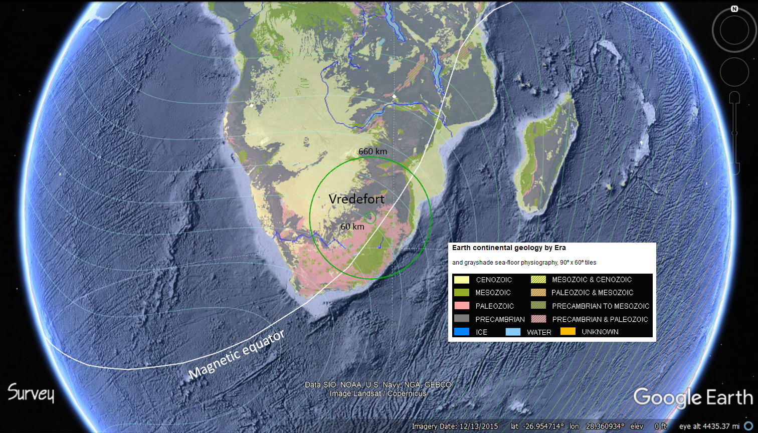

The Vredefort astrobleme and Earth's magnetic equator

Figure 5. The Vredefort crater and surrounding astrobleme is one of Earth's largest and oldest (2 billion year old) impact structures that likely imparted deep-seated mantle fractures and basic mantle melts that are part of Earth's electromagnetic dynamo as is appears to influence the location of our geomagnetic equator. Earth continental geology includes Cenozoic (yellow), Paleozoic (pink), Mesozoic (green). and Cenozoic (yellow) bedrock.

A GIF animation of Earth's magnetosphere based on a Google Earth and SketchUp Pro models

Figure 6. A GIF animation of a Google Earth KMZ file and a correlative SketchUp Pro computer model showing aspects of Earth's magnetosphere including the extraterrestrial potential field extending into space beyond the planetary surface, and the total-field magnetic intensity mapped on the surface including the magnetic equator traced in white. The 3D field is rendered in 2D space to demonstrate its asymmetry.

Four perspectives of Earth's
magnetic field including a 2D image

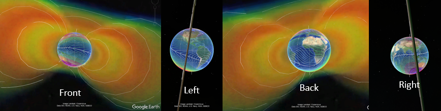Figure 7. The magnetic equator does not follow the geographic equator but dips and rises around the globe. They coincide most closely in the western Pacific and Indian Oceans. The extraterrestrial field is a 2D image aligned with the total-field intensity contours downloaded from San Diego State University in 2014. Click here for the Google Earth KMZ file shown above.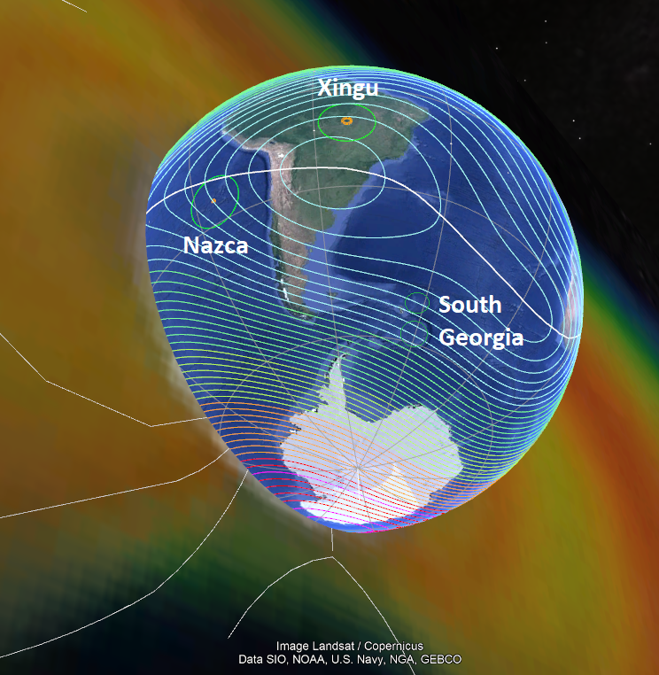

An oblique perspective of Earth's electromagnetic total-field at the planetary surface with the magnetic equator traversing the Southern region
South American magentic aspects

Figure 8. A GE view of Antarctica and the south magnetic pole relative to the magnetic equator.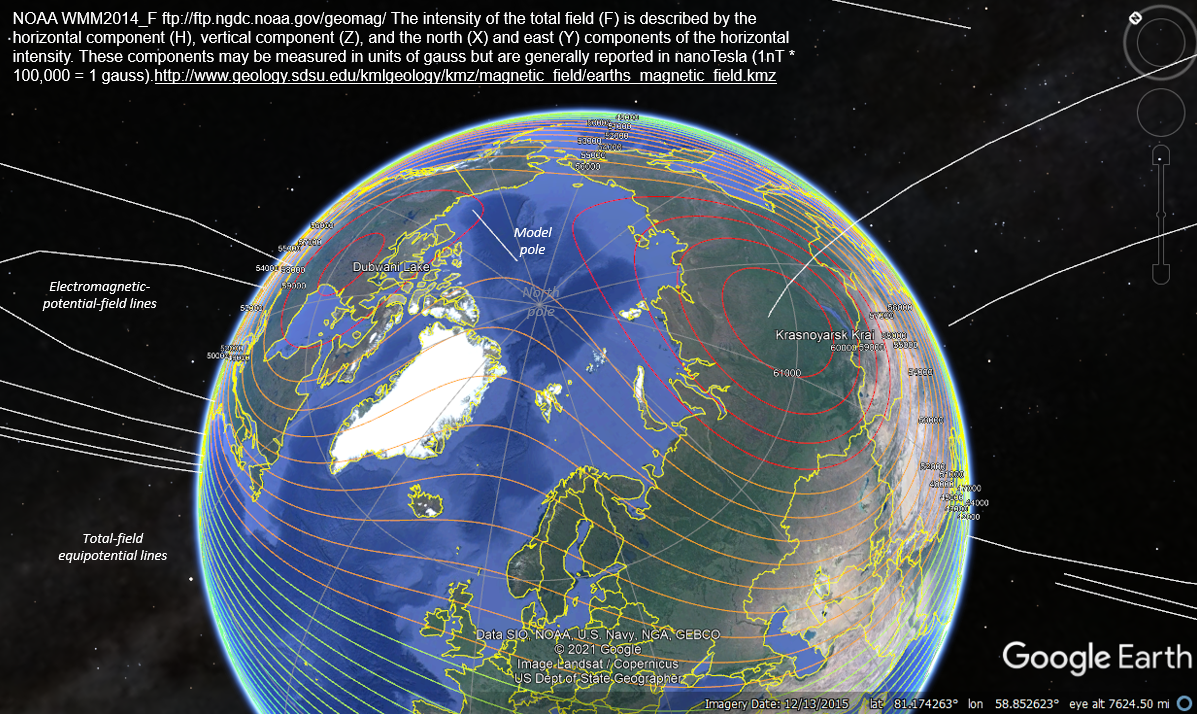

Google Earth Pro themes of Earth's total magnetic field intensity with a SUP model embedded to show the extraterrestrial, poloidal, 2D magnetic-field lines and their asymmetry with respect to the North pole.

Figure 9. Equipotential field lines (isopleths) on Earth's surface are total-magnetic field isopleths that are variously colored to emphasize the asymmetry of our electromagnetic-field with respect to Earth's spin axis. A SketchUp Pro was used to generate the 2D-polyline traces of our extraterrestrial, poloidal field component that is aligned with the surface-theme anomalies.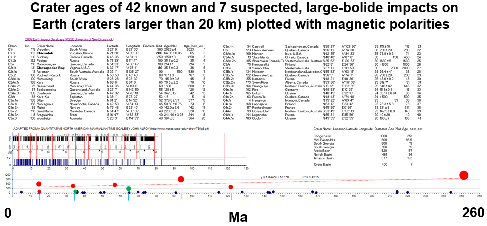

Figure 10. A Microsoft Excel scatter plot of Earth's magnetic-polarity history of the past 120 Ma including a temporal plot of the diameter of 42 known and 8 suspected impact craters probably represent a small subset of the number of actual impacts awaiting discovery. The magnetic record only covers that part of geological time represented by preserved oceanic crust.

Earth's mantle as an electromagnetic-field component, with implications for geomagnetic reversals

A conceptual, virtual, structural model is presented here that was developed to visualize physical aspects of Earth's geodynamo. The aim is to help explain the asymmetry of our geomagnetic field and mechanisms to explain polar wander and polarity reversals. The Earth model uses Google Earth and a three-dimensional computer-aided drafting (CAD) system (SketchUp Pro; SUP, rev. 2020) to visualize the major interior phase boundaries down to the solid core, the hydrodynamic outer core, and the heterogeneous mantle and lithosphere. The portrayal of mantle structures relies upon two geospatial themes and four seismic-wave tomography studies of the mantle to demonstrate its heterogeneity, and the apparent structural link having large mantle-plumes serving as major electrical components of Earth's electromagnetic armature. Earth's geomagnetic field is hypothetically a quadrapole system having one dipole fixed in alignment with the planetary spin axis, but another, poloidal dipole that migrates and wanders about the polar region through time. The former, fixed one is considered here to be the toroidal magnetic component of the quadrapole that is generated by the hydrodynamic fluid movement in the outer core, whereas the wandering one is considered here to be the poloidal dipole component arising from mantle structure. The asymmetry of the poloidal field appears to principally generated by the spinning and circulating, heterogeneous mass of electrically conductive, basic (Fe-enriched) mantle material in the form of plutons, dikes, chambers and sills stemming from mantle plumes upwelling from a slowly crystallizing core. The crust is assumed to have negligible geodynamic effects. Rather, lithospheric melt bodies are considered as electrical components of the dynamo, especially where shallow sills are electrically connected to deep-seated mantle plumes. Mantle heterogeneity and the geomagnetic field evolves through time to reflect plate tectonics and external stimuli from large-impact events. As such, polar wander and phase shifts are likely to occur following large bolide (asteroid and comet) impacts that suddenly introduce new mantle melts into the geodynamo. New, melted material assimilates into the existing system, thereby forcing the mass migration of electrons between bodies. Magnetic-field flow is spurred on by hemispherical accumulations of charged material with the hypothesis that the negative pole occurs in whichever hemisphere holds a greater volumetric mass of magnetic media.

My interest in Earth structure stems from being a structural geologist seeking answers to what forces come to bear on Earth to make mountain chains rise and large basins to form. When teaching geology at various colleges through time, the graphics that I use from various textbooks and journal articles that illustrate the dynamic interactions of our core and mantle resulting in our robust electromagnetic field haven't addressed the asymmetry of the field or the apparent link with heterogeneity of the mantle structures as gleaned from geophysical studies. After having spent many years researching the tectonic effects of hypervelocity bolide-impact strikes on terrestrial planets, I now focus here on illustrating how our geodynamo is structured to produce our life-sustaining, electromagnetic field, and what extraterrestrial forces come to bear on the process.

Over the past decade I have used Google Earth to integrate various Earth-science geospatial themes for conducting a regional neotectonic studies of the mid-Atlantic part of the North American tectonic plate (NAP). As part of that, I came across modern geospatial datasets depicting our magnetic field that are available from the United States of America (USA) National Oceanic and Atmospheric Administration (NOAA). 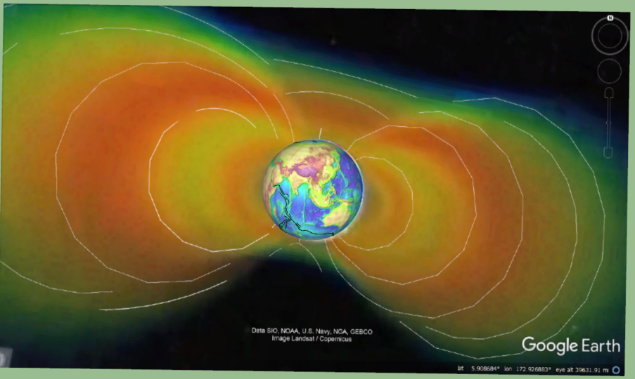Among them are magnetic-field surface-intensity themes, and four-centuries worth of mapping of our magnetic field at Earth's surface (figs. 1 to 7). Satellite remote-sensors also capture extraterrestrial aspects of our magnetosphere like that depicted in figure 5 from 2003 that demonstrates its asymmetry. The total magnetic-field theme portrayed in figures 6 to 8 is a Google Earth theme with magnetic data tagged as 2014 that was obtained from the geology department at San Diego State on a website that is no longer active as the links to the site are broken. It portrays the poloidal component of the field in accordance with the one dipole seen in NOAA's websites depiction of the field over Antarctica (fig. 1). The poloidal field is skewed with respect to the planetary spin axis and tilted towards eastern Antarctica in the south polar region (figs. 1 and 2). I was equally intrigued by the tendency for the magnetic equator to swing abruptly to and fro around the globe (figs. 5 to 8). In some place, it veers towards and away from one of the largest, confirmed, and oldest impact astroblemes in South Africa surrounding the Vredefort crater and lithospheric dome (fig. 5). These aspects prompted me to wonder what mantle structures are responsible for these peculiar effects?

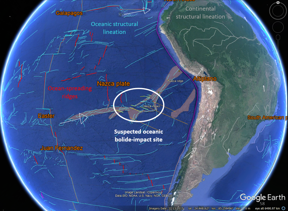
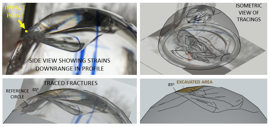
From studying impact-tectonics I have learned that large astroblemes, or impact scars on terrestrial planets commonly include large-volcanic provinces (LIPS) located in their wake where the lithosphere has been extended by oblique strikes. The large impact events appear to generate deeply penetrating mantle fractures that stimulate the melting of new mantle that if, and when connected to the existing electrical dynamo trigger electrometric field excursions and probably, occasional reversals. Moreover, consider that the total-field expression of Earth's magnetic field at the planetary surface is a sum of three different electrical components identified by phase differences, a solid inner core, a liquid outer core, and a partially molten mantle that together constitute a complex and heterogeneous electrical armature that evolves with time. The bulk of the conductive material is spread out through the mantle over vast vast regions occupied by partially melted plumes rising off the outer core (figs. 2 to 4). The volume of the mantle is over 6 times that of the outer core but only some fraction of that is likely connected electrically to the outer core (figs. 2 and 3).

A robust computer model of Earth's geodynamo was developed by University of California scientists Gary Glatzmaier (Santa Cruz), Paul Roberts (Los Angeles), and Rob Coe (Los Angeles) starting in the 1990's. Their work simulates the mechanisms and fluid motions in Earth's outer core that primarily generates Earth's geomagnetic field. Their computer simulations span millions of years, using an average numerical time step of 15 days. At the surface of the model Earth, the simulated magnetic field has an intensity, an axial dipole dominated structure, and a westward drift of the non-dipolar structure that are all similar to the Earth's. The model's solid inner core rotates slightly faster than Earth as indicated by other seismic analyses. Several spontaneous reversals of the magnetic dipole polarity also occur in the simulations, similar to those seen in the Earth's paleomagnetic record. Their model suggests that the most robust fluid flow occurs in a cylindrical, fluid column that is focused along the planetary spin axis where the hydrodynamic other core rests against the metallic (Fe>Ni) inner core, and the electromagnetic field intensity is at its greatest strength. Other geophysical work suggests that the inner core also has a layered structure reflective of the planetary spin axis that is represented here by a cylinder within the inner core (fig. 3). Both of these aspects are included in the SUP CAD model (figs. 2 and 3).

I first started modeling mantle structures using a when participating in an on-line Geological Society of America community-forum post about the structure of the Yellowstone caldera. For that, I began modeling the 3D plumbing system of Earth's mantle focused on Yellowstone's hot spot. Soon after I began adding other regional seismic-wave tomographic-study results from around the globe as 2D-profile images into a new, global model. At this time, sixteen different images are scanned and embedded in the model including some from Nolet and others (2007), French and Romanowicz (2014), Portner and others (2017), and Yuan and Romanowicz (2017). Each image was screen captured and saved as a colored-image file (*.PNG), then manually geo-registered into the SketchUp model as shown in figures 2 and 4 for various views. Some of the tomographic studies are are focused on areas of active mid-ocean spreading or subduction, but others cover hemispheric swaths of our planet and provide detailed coverage that is suitable as a basis for the geometric modeling depicted here (fig. 4). The model also includes an embedded, color-enhanced image of Earth's extraterrestrial, poloidal magnetic field stemming from the Unities States of America (USA) National Space and Aeronautic Administration (NASA) that has an image date of December 2003 (figs. 6 to 8).

Mantle structures were manually digitizing using the registered tomographic images to generate polygons around each region to extract the tomographic-defined hotter versus colder regions as mapped from surface-born seismic-monitoring stations around the globe. The alignment of the image portraying our poloidal field was embedded in the various geospatial program in an orientation coinciding with contoured maximums of the surface-based expression of the magnetic field. I assumed that this arrangement is the most logical, but the image can easily be rotated out of alignment. So one aspect of the analysis that needs further analysis is how our 3D extraterrestrial expression of the magnetic field is spatially positioned relative to the surface anomalies.

The model at this stage is incomplete and lacks many mantle details. I'm sure that there are other tomographic studies to compliment those used here that I haven't yet seen yet. Nevertheless, the embedded tomography provides a representative glimpse of the structural arrangement of the geodynamo components that constitute Earth's electrical armature. At least three distinct phase components operate including 1) the inner, solid spheroid, 2) the surrounding molten, fluid outer core, and 3) the thick, plastic heterogeneous mantle with structural heterogeneity stemming from a lifetime of bombardment, accretion, and tectonic movements. The model depicts these three different electromotive components:

1) the solid inner core, thought to be predominately an Fe-Ni alloy and a magnetic, spinning and circulating spheroid. Because the inner core rotates slightly faster than the hydrodynamic outer core it is considered a separate, electrical component. Recent studies show that the inner core has fabric, or layering of sorts that may also be aligned along the planetary spin axis. A primitive cylinder was made and placed in the center of the inner core to represent this 'battery' type of configuration (fig. 3).

2) the liquid outer core, thought to be composed of churning Fe-rich liquid with nickel, sulfur and other lesser elements that spins counterclockwise with Coriolis forcing of the outer core hydrodynamics. Any structural heterogeneity in the core would perturb the hydrodynamics accordingly. The vortices of particle motion are represented in the model using halves of Archimedes spirals that wind downward from the polar regions to the equator, because polar phase shifts on the Sun are observed to flux inward from the poles, so that is considered here to be good, representational starting point. Two sets of spirals are aligned along the spin axis, one mid-way in between the inner and outer core shells. The other set of spirals are positioned just inside the outer core shell to represent the fluid motion in the entre core in addition to that which is more focused near the planetary spin axis.

3) the ductile mantle where seismic tomography reveals lateral and vertical heterogeneity resulting from colder and warmer regions correlating to higher and slower seismic-wave speeds respectively. The slowest regions likely have the most melted material where mantle plumes rise slowly from dissolution creep to convect heat away from the solidifying core. Mineralogical phase changes occur at increasingly higher levels results in increasingly lighter material rising upward with decreasing lithostatic pressures, ultimately resulting in sill emplacement in the upper mantle (lithosphere) that feed crustal magma chambers beneath mid-oceanic spreading centers.

The mantle appears to have two separate geometric components considering that deep mantle plumes are dike-shaped plutons, and upward-migrating magma accumulates and spreads laterally near or at the base of the lithosphere forming large plutonic sills (figs. 2 to 4). Mantle plumes with the least viscosity and highest rates of dissolution creep may take on a spiral form owing to Coriolis- and centripetal- forced effects that increase toward Earth's geographic equator lying normal to the planetary spin axis.

Recent studies of our geomagnetic field demonstrate that it is a quadrapole system having two sets of dipoles occupying polar regions (Fig. 9). One seems fixed on our planetary spin axis and another wanders and drifts about at various rates (Fig. 1). It's logical that the toroidal component of the total magnetic field is the dipole aligned along the spin axis, whereas the wandering, poloidal field arises from a heterogeneous, evolving mantle. The past irregularity of Earth's poloidal-field component has a continuous, but sporadic and inconsistent record of polarity reversals reaching as far back as the splitting apart of Pangaea about 250 Ma ago (fig. 10). Total-field parameters are gained around the globe from samples and cores of oceanic crust that provide details covering the past 180 Ma. The small amount of older oceanic crust has been remagnetized so other, older records are gained from well-constrained continental samples. The total field reverses on average every 242,000 years, with a rate of occurrence that increases with time (fig. 10).

Earth's magnetic and geographic equators do not coincide. Rather, the magnetic equator dips and rises around the globe relative to the geographic equator, with excursions traversing both continents and oceans. In places it veers toward very large, bolide-impact craters (figs. 5 and 8). As seen in figure 8, the magnetic equator in the South American region dips southward to bisect the High Andes continental culmination located midway between two large, suspected impact craters having far-field tectonic strains (Nazca and Zingu River, Brazil impacts fig. 8). This suggests that the Earth's magnetic field measured at the surface is significantly influenced by lithospheric plate-tectonic process of subduction and isostasy, and that sub-plate mantle melts are also electrical components of Earth's geodynamo. It also suggests that mantle processes are largely responsible for the poloidal-field component that is in a constant state of flux owing to uniformitarian plate tectonics through time. If the toroidal component is more-or-less fixed along the planetary spin axis and quasi stable, then perhaps polarity reversals of the poloidal field spur reversals internally, that is, from the outside in.

Seismic-wave studies decrease in certainty with depth and there has been scientific debate as to whether mantle plumes rise from the core-mantle boundary (CMB), whether at all, and the exact nature of the mantle heterogeneities giving rise to the velocity perturbations. Many physical factors contribute to wave propagation among which are the percentage of melt fraction, and material-density increases with depth. The seismic tomography shows large, lateral sills of partially melted mantle where magma underplates our crust and lithosphere (figs. 2 to 4 ). It is widely know that electron transmission occurs more rapidly in wet, melted material than in it's dry counterpart. The exact nature of the mantle is therefore speculative, with uncertain volumes of liquid-and solid-fractions and depth-related mineral-phase changes resulting from gravitation compaction approaching the inner core where maximum temperatures and pressures occur. It' also certain that extraterrestrial excitement and perturbation of the mantle occurs periodically through time when large-bolide impacts impart deeply penetrating mantle fractures and faults as part of large astroblemes. Scaled-down impact experimentation shows how deeply penetrating, fractures are can be imparted from high-angle, oblique, surface impacts with penetration depths reaching one-third of the radius of a sphere. Such large events must instantly impart planetary-scale faults on terrestrial lithosphere like those seen on Mars. Such catastrophic events will produce instant melting, especially in decompressed, hinterland sectors in the wake of high-to-moderate angle, oblique impacts. Antipodal melts are also possible from high-angle impacts. When new mantled melts become electrically connected, or 'wired into' an existing geodynamo, then the electromagnetic system is perturbed and will seek to achieve a new equilibrium. The tendency of our magnetic poles to wander and flip through time could be emphasized after a punctuated, large impact event that instantly introduces new components of Earth's electrical armature and spur evolutionary changes. The flux in the the volume of electrically stimulated material will excite a total-field adaptation. Large, sustained volcanic eruptions occurring on Earth today should also then, hypothetically induce poloidal-field wander. Volcanic eruptions deplete melted material in the mantle, and therefore should promote magnetic-field drift from exhalation of electrically conductive material. Periods of rapid drift and uplift therefore coincide with periods of increased volcanic activity. These circumstances imply that plate-tectonic movements and associated melt production and solidification are processes are part of tectonic evolution of our poloidal electromagnetic field component.

The nature of Earth's magnetic field seems complex, but when broken down into various structural components, it also makes sense. Our current situation has the toroidal and poloidal dipole axes converging in the North but diverging in the South (fig. 1). The poloidal field axis is skewed toward the Indian Ocean where there are two, relatively young, sea-floor spreading triple junctions. Based on the preceding premises, it appears that there is probably a disproportionately large volume of mantle melts occupying that region, but the model compiled here isn't complete enough to do the necessary assessment of this. In summary, it's uncertain whether this three-component model for our geodynamo will prove to be accurate. I stumbled onto this solution in the course of assembling worldwide, geospatial data, and I find it remarkable that there are no precedence for these hypotheses. As such, they may be novel, and if so, I expect them to smolder for a long period before catching fire. In the end, I simply hope that these concepts prove insightful for developing a quantitative basis.

French, S. W., and Romanowicz, B. A., 2014, Whole-mantle radially anisotropic shear velocity structure from spectral-element waveform tomography: Geophysics Journal International, v. 199, p. 1300-1327

Portner, D. E., Beck, S., Zandt, G., and Scire, A., 2017, The nature of subslab slow velocity anomalies beneath South America, Geophysical Research Letters., v. 44, p. 1-9. doi:10.1002/2017GL073106.

Roberts, P. H. and Glatzmaier, G. A., 2001. The geodynamo, past, present, and future: Geophysics, Astrophysics, and Fluid Dynamics. vol. 94, p. 47-84

Stephenson, J., Tkalčić, H., & Sambridge, M., 2021, Evidence for the innermost inner core: Robust parameter search for radially varying anisotropy using the neighborhood algorithm. Journal of Geophysical Research: Solid Earth, 126, e2020JB020545. https://doi.org/10.1029/2020JB020545

Yuan, K., and Romanowicz, B., 2017, Seismic evidence for partial melting at the root of major hot spot plumes: Science, v. 357. p/ 393-397.